Impact modeling and sustainability assessment

After defining the evolution of air transport via dedicated models, specific models evaluate the associated impacts, and then compare them with limits via a sustainability assessment.

Impact modeling

In the following, the models used for estimating the impacts induced by air transport are described. Currently, the majority of impact modeling concern environmental impacts.

Emissions and climate impacts

CO₂ emissions

Based on the modeling of the air transport system through a Kaya decomposition, the estimation of the evolution of CO₂ emissions is simple by multiplying the different factors. In addition, a coefficient corresponding to other life cycle emissions (excluding combustion and fuel production) can also be applied, but it only represents a few percent of the aviation environmental impacts [PMBC+20].

Non-CO₂ emissions

For estimating non-CO₂ emissions, the concept of Emission Index (EI) is used. They make it possible to obtain different emissions (NO_x, SO_x…) depending on fuel consumption (or CO₂ emissions). Values for fossil kerosene from [LFS+21] have been used and are provided in Tab.1. The values can be adapted for alternative energy carriers.

Emission	Value	Unit
CO2	3.15	kgCO2/kgfuel
H2O	1.23	kgH2O/kgfuel
NOx	15.1	gNOx/kgfuel
Aerosols (soot)	0.03	gBC/kgfuel
Aerosols (sulfur)	1.2	gSOx/kgfuel

Tab.1 Emission Index for fossil kerosene combustion.

Based on these data, the estimation of the climate impact of aviation is achieved by the calculation of the ERF (Effective Radiative Forcing), which is based on the use of coefficients for the different impacts. These are obtained through an analysis of the data from [LFS+21] and are summarized in Tab.2. CO₂ emissions are cumulative: therefore, at first order, the coefficient to estimate the ERF must be applied on the cumulative CO₂ emissions. The impact of the other emissions is estimated from the annual emissions. Finally, the impact of contrails is assumed to be correlated with the total annual distance flown.

Climate impact	Value	Unit
CO2 (cumulative)	0.88	mW/m2/GtCO2
H2O	0.0052	mW/m2/TgH2O
NOx	11.55	mW/m2/TgN
Aerosols (soot)	100.7	mW/m2/TgBC
Aerosols (sulfur)	-19.9	mW/m2/TgSO2
Condensation trails	1.058.10-9	mW/m2/km

Tab.2 Coefficients for estimating the ERF of aviation climate impacts.

Using the data and taking into account CO₂ and non-CO₂ effects, aviation (including private and military) generated 3.8% of the effective radiative forcing between 1750 and 2018 and commercial aviation is responsible for 5.1% of the increase in effective radiative forcing over a more recent period (2000–2018), compared to global ERF estimated in the IPCC AR6.

Lastly, equivalent emissions can be estimated to simplify the comparison with CO₂ emissions, but also to estimate the impacts on the temperature evolution in a second step. Multiple metrics are available in the scientific literature to estimate them [APF13, SFHS05]: GWP, AGWP, GTP, AGTP, etc. GWP is the most known and used metric, often used with a 100-year time horizon. However, this metric is limited for representing the evolution in terms of temperature for Short-Lived Climate Pollutants (SLCPs) [LCPA20], which is the case for aviation non-CO₂ effects. As a consequence, an alternative metric is used here. GWP* is an improved climate metric developed recently [ASF+18, CLA+19, CFFS20], one of the major interests of which is to better evaluate the effect of SLCPs. It allows to estimate the equivalent emissions in CO₂-we for a better match with the evolution in temperature (warming equivalent). In this sense, it thus represents a simplified climate model compared to other more complex climate models that may require long computation times [MN22]. Compared to GWP, it does not only take into account the absolute value of the emissions but also the variation of the emission rate. The following equation allows estimating the equivalent emissions, noted \(E_{CO_2\text{-we}}\), of a gas \(G\) for a time horizon \(H\), as a function of the absolute emissions \(E_G\) and the variation of emissions \(\Delta E_G\) over a period \(\Delta t\). The parameters \(r\) and \(s\) depend on the gas and represent the influence of cumulative or short-term effects.

\(E_{CO_2\text{-we}} = \text{GWP}_H ~ \left(r ~\frac{\Delta E_G}{\Delta t}~H + s~E_G \right)\)

This equation can be modified to be used for aviation non-CO₂ effects, based on assumptions from [ASF+18, LFS+21], with in particular \(r=1\) and \(s=0\). As a consequence, the following equation is used with \(E_{CO_2\text{-}we}\) the equivalent emissions of a non-CO₂ effect for a given year, \(\Delta F\) the corresponding variation of the ERF over a period \(\Delta t\) of 20 years (smoothed over 5 years to better represent global trends), a time horizon \(H\) of 100 years and the absolute global warming potential of CO₂ over 100 years \(AGWP_H\) of 88 yr.mW/m²/GtCO₂.

\(E_{CO_2\text{-}we} = \frac{\Delta F}{\Delta t} \frac{H}{AGWP_H}\)

Temperature estimation

Based on the knowledge of the CO₂ emissions and non-CO₂ effects via equivalent emissions, it is possible to estimate the temperature increase due to air transport \(T_{k}\) for the year \(k\). For this purpose, the following equation is used with \(T_{2019}\) the temperature increase from air transport in 2019 (from [GGRGronstedt+21]), \(E_{CO_2, k}\) the annual CO₂ emissions and \(E_{CO_2\text{-}we, k}\) the annual equivalent emissions for non-CO₂ effects using GWP*. The value of the TCRE (Transient Climate Response to cumulative carbon Emissions) depends on climate model settings, with median estimates on the order of 0.45°C/1000GtCO₂. However, it is also possible to estimate the temperature increase from air transport using dedicated climate models for more accurate results.

\(T_{k} = T_{2019} + TCRE ~ \sum_{i=2020}^{k} (E_{CO_2, k} + E_{CO_2\text{-}we, k})\)

Energy resources

The description of the energy carriers envisaged for air transport makes it possible to estimate the quantities of fuels to be used (embarked energy), but also the quantities of energy required to produce them using conversion efficiencies. The quantities of biomass and electricity consumed are then directly calculated. The selectivity of the pathways producing these energy carriers, defined as the proportion of kerosene in the fuel output (usually measured by energy), can also be taken into account. It allows to estimate the amount of energy that has to be used to produce kerosene and other outputs. However, in general, an allocation of consumption is made to other outputs for estimating the “real consumption” due to kerosene (which means that selectivity is not taken into account).

Economic

The current cost models implemented in AeroMAPS are described in this section. A recap of the energy cost models is first provided. Alternative energy cost models were presented in detail in [SPlanesD+23], with a model taking as an input each fuel pathway annual energy consumption to derive annual energy expenses and the required investments chronology for the energy sector. A direct operating cost model adapted to AeroMAPS was recalibrated in [SDPlanesL23] and adapted to AeroMAPS in [SDPlanes+23].

Alternative energy cost model

As mentioned in the air transport modelling section, three biofuel production pathways are modelled within AeroMAPS: Hydroprocessed Esters and Fatty Acids (HEFA), Fischer-Tropsch (FT), and Alcohol-To-Jet (AtJ). Regarding their production costs, three main drivers are identified by the literature [dJ18, Pav19]: the capital required to build a conversion plant (Capital Expenditures – CapEx), and the operational expenditures, in which we can distinguish between the supply of energy to be converted, referred to as feedstock in the following, and other expenses (personnel, various inputs, maintenance, etc.), referred to as OpEx. Despite large new scale-up plans for theses fuels like ReFuelEU, these are still niche markets, meaning that no mature price exists for the trade of these biofuels. A proxy metric used is the Minimal Fuel Selling Price (MFSP). It is the fuel selling price at which the fuel production project has a null Net Present Value (NPV). This value is the difference between the expenses and the revenues from a project during all its lifespan and considering the time value of money: a large investment immobilized in a project whose revenues occurs much latter represents an opportunity cost. It is considered by the discount rate r, which discounts future cash flows. Overall, the MFSP can be determined using the following equation, where \(CAPEX_t\) are the capital expenditures at year \(t\), \(OPEX_t\) the operational expenditure on the same year, feedstock expenditures \(FEED_t\) excluded. \(P_t\) is the quantity of fuel produced. One can see that MFSP is indeed the minimal constant price at which the fuel should be sold to ensure the project profitability.

\(MFSP = \frac{\sum_{t=0}^{N-1}\frac{CAPEX_t}{(1+r)^t}+\frac{OPEX_t}{(1+r)^t}+\frac{FEED_t}{(1+r)^t}}{\sum_{t=0}^{N-1}\frac{P_t}{(1+r)^t}}\)

In AeroMAPS, the biofuel MFSP were directly taken from a literature review [dJ18, IRE21, Pav19], and the CapEx values were also taken or estimated by reversing the previous equation under standard financial assumptions. It allows to estimate the annual investment required in each production pathway besides computing the MFSP of the fuel used. Once this MFSP is known, computing the extra cost for the airlines is straightforward by subtracting the cost incurred by purchasing a similar amount of fossil kerosene, assuming both fuels are perfect substitutes. A last metric is used: the carbon abatement cost \(CAC\). It combines the MFSP of a fuel with its environmental benefit, which is modeled in the environmental impact module of the tool. For the biofuel \(i\), it is the ratio between the cost difference \(\Delta_C\) to the fossil reference and the emission factor difference \(\Delta_{EF}\) with the same fossil reference, as shown below. It is used with €/tCO2 as a unit and allows to evaluate the economic efficiency of various alternative fuels. The concept can be generalized to any decarbonization measure.

\(CA_i =\frac{\Delta C}{\Delta EF}= \frac{C_i-C_{fossil}}{EF_{fossil} -EF_{i}}\)

Both electrofuels and hydrogen are modelled in an equivalent way as biofuels. Schematically, hydrogen can be either used directly, burned in a gas turbine or as a fuel of a redox reaction in a fuel cell, or indirectly through the production of a synthetic kerosene. In the latter case, it is combined with CO2 in a Fischer-Tropsch (amongst others) pathway to produce a drop-in fuel. The cost modelling follows a similar process as before, but the MFSP equation is this time directly used as an explicit MFSP model. Besides, it is adapted to index the hydrogen price on the yearly energy price (equivalent of feedstock for biofuels). For hydrogen production, electrolysis, steam methane reforming and coal gasification are modeled. Carbon Capture and Storage can be added to the fossil pathways. Reference technological values on CapEx, OpEx and efficiencies are taken from [Age21, PIK22, UdfB21]. When hydrogen is directly used, the cost of other production steps has to be added to its total cost. For instance, for volume reasons, its use in aircraft could require its liquefaction, and the supply chain (transport, storage and refuelling) would be modified as well. Those costs are also modelled in the module. The carbon abatement cost is thus computed using the equation above as well. The economic modelling of electrofuels is similar, though a last cost component should be accounted for: the CO2, whose direct air capture is a major cost driver.

Lastly, the expenses for kerosene are also modelled according to its market price specified by the user. By default, it is set to its average historical price (0.41€/L). Note that alternative fuel market is not modelled. MFSPs are therefore a lower bound of their potential prices. Kerosene production CapEx (plant renewal and/or expansion) is not modelled so far.

The user is also able to specify a uniform carbon tax, that is applied to all energies (fossil, biofuel, e-fuel and hydrogen) using their emission factors. Two metrics are computed: a supplement to the previous MFSP and the total expenses (or fiscal revenue) for each pathway using the associated consumption as well. By default, a fictional carbon tax implementing in full the French Value for Climate Action [Qui20] is used.

Direct operating cost (DOC) model

Airline costs can be split into two informal categories: the costs directly related to operating an aircraft and those related to general business operations named non-operating costs (administration, sales, …). For the former category, they can be further split between Direct Operating Cost (DOC) and indirect operating costs. Like non-operating costs, indirect operating costs are not directly linked to the aircraft operation but rather to passenger service. With a simplified approach, there are five main categories in the DOC: capital (owning an aircraft), crew, fuel, maintenance, and fees/taxes. In AeroMAPS, a further simplification is made by using three categories: fuel (or energy), non-energy and carbon taxes.

Explicit direct operating cost models are presented in [RSSS16], on a per flight hour basis. These models depend directly on the aircraft characteristics. They were recalibrated using United States Bureau of Transportation Statistics data and adapted to a per flight basis in [SDPlanesL23]. Since AeroMAPS uses a global top-down approach to model flights by simulating the evolution of the Revenue Passengers Kilometres (RPK) for different markets rather than aggregating many flights, the direct use of these cost models would be of little interest. Therefore, average values for selected aircraft and distance categories were extracted from the results of [SDPlanesL23] based on the full simulation of a year (2019) of US airlines flight. Note that it introduces an obvious geographical bias, some costs being widely dependent on the country or the airline (crew, capital structure, age of the fleet, …). However, the lack of reliable detailed financial data to recalibrate the cost model made this limitation necessary.

For non-energy DOC, average costs per aircraft type (regional jet, single-aisle aircraft on short and medium-range routes and long-range), per Available Seat Kilometre (ASK) are used as a starting point. Their evolution is modelled using two different possibilities, like aircraft efficiency. Either simple models implement an annual, category-wide evolution in non-energy DOCs, or bottom-up fleet renewal models are used with discrete DOC values for each aircraft introduced.

Concerning the fuel DOC, it is directly linked to the energy cost module described before. Indeed, the fuel cost is simply obtained by multiplying each aircraft category energy consumption by the average fuel price from the energy cost module. For the moment, each aircraft type in the drop-in fleet is considered to use a blend of all the pathways of the scenario (for example, a situation in which a new generation aircraft uses 100% SAFs while the older generation uses only fossil kerosene is not considered).

Manufacturing cost model

This model is under implementation, but a beta version is described in [SDPlanes+23].

Sustainability assessment

In the following, the methodologies used to assess the environmental sustainability of scenarios are presented, based on estimates of induced environmental impacts. Only climate and energy issues are considered. Indeed, these two environmental issues are the most impacting when considering air transport (see for instance [Planes22]).

Climate sustainability

Climate sustainability assessment can be performed using various methodologies. For example, carbon budgets. It is an interesting concept used by the IPCC in the context of global warming mitigation strategies. It is defined as the maximum remaining cumulative CO₂ emissions that can be emitted to limit the temperature increase below a certain value (for example +1.5°C). For instance, Tab.3 summarizes estimates of carbon budgets for different temperature targets. The emissions considered are net emissions: they are the difference between gross anthropogenic CO₂ emissions and anthropogenic carbon sinks. Cumulative CO₂ emissions and mean temperature increase are linked by a quasi-linear relationship, which facilitates the estimation of carbon budgets [MGSZ09]. Therefore, the use of carbon budgets allows for example to simply evaluate the relevance of transition scenarios to reach climate objectives based on their CO₂ emissions alone [FAR+14].

Temperature [°C]	17th	33rd	50th	67th	83rd
1.5	900	650	500	400	300
1.6	1200	850	650	550	400
1.7	1450	1050	850	700	550
1.8	1750	1250	1000	850	650
1.9	2000	1450	1200	1000	800
2.0	2300	1700	1350	1150	900

Tab.3 Estimates of carbon budgets depending on TCRE percentile according to IPCC AR6 (in GtCO₂).

However, these carbon budgets are defined globally and not by country or sector (like aviation). In the following, a method which can be applied to aviation CO₂ emissions is proposed. This later is also extended to include non-CO₂ effects using two solutions.

CO₂ effects

First, a global gross carbon budget \(GCB\) is considered. As a reminder, it is defined as the sum of a net carbon budget and a CDR (Carbon Dioxide Removal) capacity (afforestation, BECCS, DACCS…). It is assumed that this budget will be entirely consumed by 2100. This constraint is expressed in the following equation via cumulative emissions, considering \(E_{CO_2,k}\) emissions for year \(k\) from 2020.

\(GCB = \sum_{k=2020}^{2100} E_{CO_2,k}\)

An infinite number of trajectories for CO₂ emissions can satisfy this constraint. In the following, a simplified model of emissions decay at a fixed annual rate \(x\) is considered. The previous equation can then be written as the following one. This is a geometric series which can then be expressed more simply. This equation can then be solved implicitly to determine the annual rate of decrease of emissions \(x\).

\(GCB = \sum_{k=2020}^{2100} E_{CO_2,2019}~(1-x)^{k-2019} = E_{CO_2,2019}~ \frac{(1-x)-(1-x)^{82}}{x}\)

Here, the scope of the scenario studies is limited to 2050. Therefore, the following equation is used to determine the adjusted global gross carbon budget to 2050 \(GCB_c\).

\(GCB_c = E_{CO_2,2019}~\frac{(1-x)-(1-x)^{32}}{x}\)

Finally, it is necessary to allocate a share of this carbon budget to aviation. Thus, the carbon budget for aviation (by 2050) \(GCB_A\) is simply calculated using the following equation via an allocated share \(F\).

\(GCB_A = F~GCB_c\)

The choice of the share allocated to the aviation sector is a political one and may involve multiple criteria (technical, economic, societal, etc.). Discussions on this allocation are proposed in [DFG+22]. An interesting reference value is the recent contribution of aviation to CO₂ emissions (also called grandfathering approach). For example, it is 2.6% on the perimeter of commercial aviation considering global CO₂ emissions [DFG+22]. This value can be interpreted as the share that would be allocated to the aviation sector under a non-differentiated approach where all sectors reduce their emissions at the same rate. Allocations below or above this value can also be considered. However, allocating a larger share mechanically requires other sectors to reduce their emissions faster than the average to meet the global carbon budget. This type of trade-off may require multi-sectoral approaches, as for example proposed in [ScienceBTInitiative15]. In this scenario, cumulative direct CO₂ emissions from aviation would represent 3.4% of the considered carbon budget of 1055 GtCO₂ over the period 2011–2050.

Therefore, the climate sustainability of a scenario (regarding CO₂ emissions) can be assessed by comparing the cumulative CO₂ emissions with the allocated carbon budget for aviation. If the cumulative emissions are less than or equal to the carbon budget, the climate target is met.

CO₂ and non-CO₂ effects

For assessing the sustainability of aviation climate impact, a first solution is to directly compare the temperature increase from air transport to a climate objective (via an allocation or an absolute target) which is for instance performed in [GGRGronstedt+21, KlowerAL+21].

Another solution is to extend the previous approach in order to maintain a methodology similar to that used for CO₂ emissions. So-called equivalent carbon budgets are then calculated. For this purpose, a global equivalent gross carbon budget \(EGCB\) is calculated via the following equation, which has been adapted from simplified models for estimating carbon budgets described in [RFK+19]. The \(T_{non-CO_2}\) term depends on the temperature objective considered: it is for example equal to 0.1°C for a +1.5°C target and to 0.2°C for +2°C.

\(EGCB = GCB + \frac{T_{non-CO_2}}{TCRE}\)

The same approach as for CO₂ emissions is then used to define an equivalent carbon budget for aviation. Allocation rules must also be defined. The reference value considered this time is 5.1%, on the perimeter of commercial aviation, over a recent period and including global CO₂ emissions and non-CO₂ effects [DFG+22].

Therefore, as before, the climate sustainability of a scenario (for all effects) can be assessed by comparing the cumulative equivalent emissions with the equivalent carbon budget calculated for aviation. As introduced previously, the equivalent emissions are also calculated using the GWP^* climate metric. The total cumulative equivalent emissions are thus the sum of the cumulative emissions of CO₂ and the sum of these annual equivalent emissions for each non-CO₂ effect from 2020 to 2050.

Energy resource sustainability

The assessment of energy resource sustainability is based on an approach similar to the one presented for climate issues. This time, rather than comparing cumulative emissions to carbon budgets, the energy consumption of a scenario is compared to available energy resource budgets. Only biomass and electricity energy resources are studied in this work. To simplify the comparisons, the availabilities are checked in 2050. A more comprehensive approach would be to check the availability of energy resources on an annual basis.

In the same way as for carbon budgets, an arbitrary allocation of energy resources for aviation is assumed. The choice of a reference value can, for example, be based on the contribution of the sector to world energy or oil consumption (of the order of 2 to 3% or 7 to 8%). Thus, a scenario can be considered sustainable from an energy point of view if the consumption of energy resources in 2050 does not exceed the energy resource budget considered.

In the following, some examples of reasonable values are proposed.

Biomass availability

The estimation of the available biomass at the global level is complex and depends on several criteria. In this work, a statistical analysis of IRENA (International Renewable ENergy Agency) data is performed. The resource categories described for the biofuel pathways are used. The results are given in Tab.4. The lower and upper fences are determined to exclude extreme values (outliers).

Resource	Lower fence	Q1	Median	Q3	Upper fence
Waste	9	10	12	20	27
Agricultural residues	10	30	57	103	204
Forest residues	5	15	17	39	59
Energy crops	8	37	63	109	217
Algae	5	8	15	31	50
Total	37	100	164	302	557

Tab.4 Global biomass availability (in EJ) scenarios to 2050.

The estimates in Tab.4 are refined using an analysis of the references [SMB17, SMS+18] to obtain detailed results for different resources. Concerning waste, used cooking oil represents a deposit of about 1 EJ, the rest being municipal solid waste. Energy crops are divided into 63% lignocellulose, 9% vegetable oils and 28% sugar or starch-based materials.

The results obtained are consistent with [SBG14] which concludes that likely estimates are less than 300 EJ. Similarly, the results by resource type are of the same order of magnitude as those given in [OMalleyPS21].

Electricity availability

Concerning electricity at the global level, the estimation is also complex due to technical, economic or political factors. Multiple availability scenarios are proposed by academic, industrial and institutional actors. Several scenarios are thus represented on Fig.1, with the estimation of the availability but also of the emission factor of the electricity mix. It is interesting to note the reference point in 2019 and the wide dispersion of the scenarios. Moreover, all the scenarios forecast an increase in electricity production and a decrease in the emission factor. For comparison, the emission factors at the global level for low-carbon production means are lower than 50 gCO₂-eq/kWh, with values of the order of 10 gCO₂-eq/kWh for wind or nuclear power [SQP+13]. In this work, the electricity energy resource budget is therefore based on these different estimates.

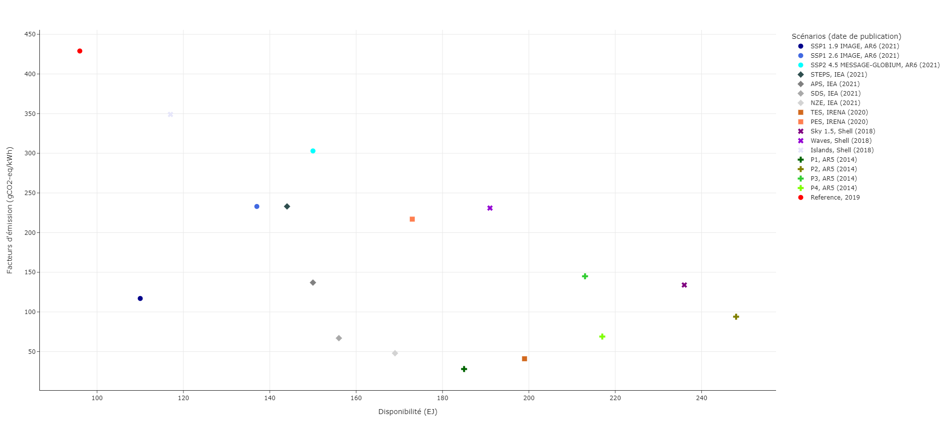
Fig.1 Global electricity production scenarios to 2050.