Use of the graphical user interface#
This page guides the user through the handling of the AeroMAPS Graphical User Interface (GUI). It is recommended to use it on a computer. First, a tutorial is provided for understanding the use of the GUI. Then, the default settings used on the GUI are provided (for details concerning the models, refer to the dedicated sections of this documentation). Finally, a procedure for using the GUI locally is presented.
Tutorial#
The AeroMAPS GUI is composed of 3 tabs:
Simulator which is the integrated simulator to directly simulate prospective scenarios for air transport ;
Data which allows to visualize data and retrieve them in CSV format in order to post-process them ;
About AeroMAPS which provides brief information, explanations and documentation about the framework.
Navigating on the tool and on the explanatory tabs is quite intuitive by clicking on the corresponding tabs. To adjust the size of the tool to the size of his screen, the user can use the zoom (out) functionalities of his browser. The display language can be chosen : English or French (coming soon).
To use the AeroMAPS simulator, the user must select the Simulator tab. Two distinct blocks then appear on the user’s screen (see the following figure).
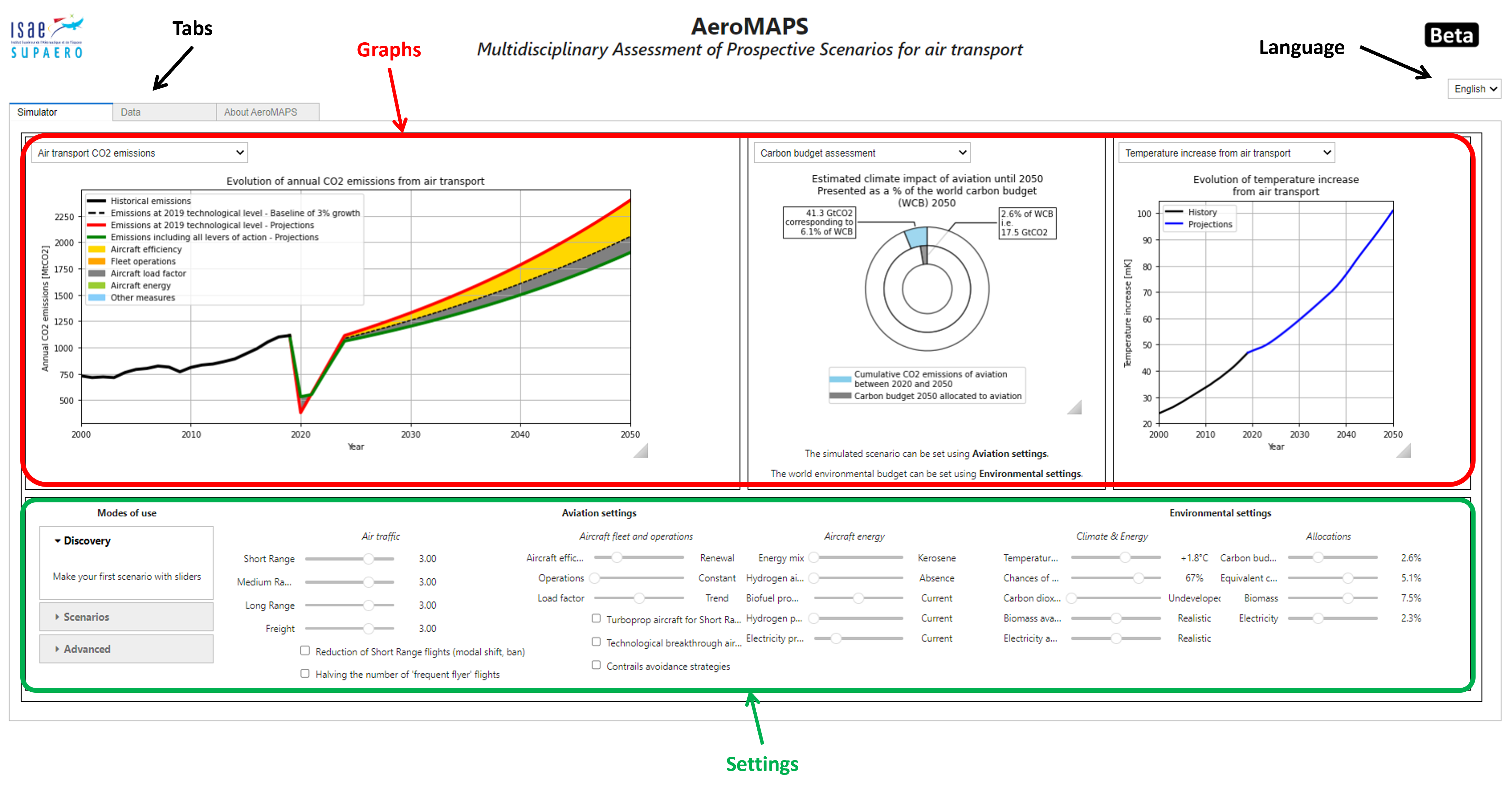
On the one hand, three different graphs are available in the upper part of the screen, with the possibility of selecting specific figures using drop-down menus. A first graph allows plotting CO2 emissions or effective radiative forcing from aviation. A second one provide figures concerning the assessment of the sustainability of a scenario, for instance in terms of climate. A last graph represents a set of figures for analyzing scenarios more deeply.
On the other hand, a set of sliders is available in the lower part of the screen to set scenario parameters. To facilitate the handling of the tool, the user can use three distinct modes of varying complexity. In the Discovery mode, the user directly uses sliders: this mode provides a good understanding of the sensitivities of the main levers of action. In the Scenarios mode, the user displays scenarios that have already been defined and parameterized: this is the easiest mode to use which only allows analyzing scenarios. Finally, the Advanced mode, not directly available on the GUI, links to the AeroMAPS GitHub to be able to manipulate in detail the AeroMAPS framework using Jupyter Notebooks.
NOTE: Additional information on the different sliders on the Discovery mode is provided by hovering the mouse over them (tooltip).
To illustrate the handling of AeroMAPS, an animation is given below. In this animation, the user tries out different AeroMAPS functionalities: moving on the tabs, using different simulator modes, displaying different figures, setting scenario parameters.
Reference settings#
The different default settings for using the interface are detailed in the following, both for the Discovery mode and the Scenarios mode. To access the detailed data, the advanced user can directly check the values into the source code in the GUI section.
Discovery mode#
In this mode, the user can play with different sliders corresponding roughly to the AeroMAPS architecture. On the one hand, aviation settings are provided for modeling the air transport evolution through air traffic, aircraft fleet and operations, and aircraft energy. On the other hand, environmental settings are given via climate and energy assumptions and allocations choices.
Air traffic#
The user can first make assumptions on the evolution of air traffic. By default, a modeling of Covid-19 epidemic is included. It significantly disrupted global air traffic in 2020 and its consequences are likely to disrupt global traffic for several years. To take account of this epidemic, a 66% decline in air traffic in 2020 compared with 2019 and a return to the 2019 level by 2024 according to IATA are considered. This modeling also takes into account the decrease aircraft load factor in 2020, which has dropped to 65.2%, against 82.4% in 2019. Similarly, due to the fact that more efficient aircraft did not fly, overall fleet performance has dropped (energy intensity per ASK increased by 30.5%). Thus, due to these factors, a paradoxical situation is obtained. Indeed, this drop in performance leads here to an increase in emissions compared to those expected without modification of the efficiency levers of action.
Overall, the user can directly define mean air traffic growth rates on the period 2020–2050 for the four considered markets in the model: passenger short-range, passenger medium-range, passenger long-range and freight. By default, these values are fixed to 3% per year, i.e. values close to aviation industry’s projections [AirTransportActionGroup21].
Moreover, an option is proposed for modeling a reduction of short-range flights, which could be induced by modal shift (substitution with rail traffic for instance) or political air route ban. Therefore, an illustrative reduction of 50% of short-range flights is integrated. The implementation is based on a logistic function with a starting year in 2025 and a duration of 5 years.
Lastly, a last option is provided for studying societal aspects on the distribution of flights, based on [GosslingH20]. The authors show that only 11% of the world’s population flies, and only between 2 and 4% go abroad. Moreover,’frequent flyers’, about 1% of the world’s population, who fly an average of 56,000 km per year (about 3 long-range trips), are responsible for about 50% of aviation CO2 emissions, taking into account their number of flights but also the more frequent use of upper classes. Therefore, an option for halving the number of flights of these people is present, by reducing by 25% the traffic (via RPK) for each market. The implementation is based on a logistic function with a starting year in 2025 and a duration of 5 years.
Aircraft fleet and operations#
The user can improve the aircraft fleet and operations.
For that, a first slider allows introducing new aircraft into the fleet, which can be improved in terms of propulsion (more efficient engines), aerodynamics, mass, systems or breakthrough architectures. Whereas an option corresponds to an efficiency improvement based on a basic fleet renewal with the current more efficient aircraft, others allow integrating future more efficient architecture. A “trend” option includes a deployment similar to the previous one in terms of efficiency gains, Entry-Into-Service (EIS) year and fleet renewal rate, which corresponds to an annual efficiency gains of around 1%. A more “optimistic” solution considers the same assumptions with an accelerated fleet turnover. Finally, an “ambitious” option takes into account the introduction of very efficient aircraft.
Another slider represents the improvements in terms of operations through flight trajectories, air traffic management, formation flights or ground operations evolution. The user can choose efficiency gains more or less ambitious, from 0% to 12% by 2050. For each option, the settings corresponding to the deployment of these solutions are similar, i.e. a duration of deployment of 20 years (for reaching 98% of the total gains) from 2025.
The user can also set the evolution of the mean aircraft load factor in 2050. The default setting corresponds to a trend estimation of 89% by 2050, but other settings are available: 82.4%, 85%, 92%, 95%. The more pessimistic option corresponds to 2019 value, whereas the more optimistic one is probably be hard to reach for all the fleet even if some airlines have already reached this value in 2019.
Lastly, two options can be activated by the user. On the one hand, the use of turboprop aircraft on short-range market is proposed for reducing fuel consumption (but at the cost of lower flight speed). The considered EIS is 2030 with a 20% reduction in fuel consumption per ASK compared with turbofan engines. On the other hand, another option consists of dedicated operational measures for avoiding contrails. It is assumed a contrails climate impact reduction of 59.4% for a fuel overconsumption of 0.014%. The implementation is based on a logistic function with a starting year in 2030 and a duration of 15 years.
Aircraft energy#
The user can define the energy that will be use by the future aircraft fleet. Here, only three main alternative fuels are considered as alternative energy carriers.
On the one hand, the user can define the future mix of drop-in fuels, i.e. fuels that can (almost) directly replace fossil kerosene such as biofuels and electrofuels. A default option corresponds to the exclusive use of fossil kerosene. Then, a biofuel option represents the exclusive use of biofuels by 2050, with a progressive replacement of fossil kerosene by biofuels from 2025. A similar one represents the exclusive use of electrofuels by 2050, with a progressive replacement of fossil kerosene by electrofuels from 2030. Finally, the ReFuelEU option corresponds to the implementation of the blending mandates at the european level, considering only drop-in fuels. This option considers the deployment of biofuels from 2025 and electrofuels from 2030, with a final mix in 2050 of 35% biofuels, 35% electrofuels and 30% fossil kerosene.
On the other hand, the user can also introduce hydrogen aircraft into the fleet. This type of aircraft also requires dedicated architectures (unlike drop-in fuels) which will probably be limited to low ranges for structural reasons (low gravimetric index for hydrogen tanks). As a consequence, the settings used are based on the fleet renewal values. The default option does not consider the use of hydrogen aircraft. A limited introduction considers a late EIS in 2040 only for 50% of the short-range market, whereas a moderate one considers a forecast EIS in 2035 for the same market. Finally, an ambitious option includes the large deployment of hydrogen aircraft for all the short-range market from 2035 and 50% of the medium-range market from 2040.
Concerning the production of these alternative fuels, the user can make assumptions on biofuel emission factors, hydrogen production pathways and electric mix. For biofuels, the default value corresponds to the median value for HEFA pathway (20.7 gCO2-eq/MJfuel), which is the most used pathway currently. A high-carbon value of 52.2 gCO2-eq/MJfuel (corresponding to AtJ pathway) and a low-carbon value of 7.7 gCO2-eq/MJfuel (corresponding to FT pathway) can also be chosen. These values can be compared to the value of 88.7 gCO2-eq/MJfuel for fossil kerosene (including production emissions). Concerning hydrogen production, four options are proposed: a current one which is mainly a mix between steam reformation of methane or the gasification of coal, two other ones based on steam reformation of methane only with or without carbon capture and storage (CCS), a last one based on electrolysis whose emission factor depends on electricity mix. Finally, the electric mix can be assumed as more or less low-carbon, with a default option corresponding to the current world grid electric mix (429 gCO2-eq/kWh). In addition to an illustrative option with high-carbon intensive electricity (1100 gCO2-eq/kWh), two examples of power grid can be considered, assuming a transition reaching medium- (240 gCO2-eq/kWh) or low-carbon (70 gCO2-eq/kWh) final mixes by 2050. Moreover, a last option corresponds to dedicated electricity from renewable (20 gCO2-eq/kWh) from today.
Climate & Energy#
The user has to set environmental assumptions.
On the one hand, several sliders are available concerning the climate settings. First, the user has to choose the temperature target for the assessment of the climate sustainability (between +1.5°C and +2.0°C, corresponding to extreme values from Paris Agreement), as well as the chances of success for achieving this climate target. This last value corresponds to the percentile considered for the TCRE coefficient used in climate sciences (for instance for estimating net carbon budgets). The default setting represents SBTi targets (+1.8°C with 67% of success). Moreover, the user can assume Carbon Dioxide Removal (CDR), which corresponds to negative emissions through for instance reforestation, bioenergy with capture and carbon storage (BECSS) or direct air capture with carbon storage (DACCS). By default, this option is disabled but the user can select values obtained from a statistical analysis of IPCC AR6 (Q1, median, Q3). The cumulative CDR over the period 2020–2100 ranges between 285 GtCO2 and 733 GtCO2 with a median value of 527 GtCO2. It allows estimating gross carbon budget.
On the other hand, two sliders are available concerning the energy settings. Indeed, the user can make assumptions on biomass and electricity availability in 2050. The biomass can be waste, agricultural or forrest residues, energy crops and algae. The default value of 164 EJ of biomass available in 2050 corresponds to a median value obtained from a statistical analysis of scientific papers and reports. The other values correspond to other statistical characteristics, ranging from 37 EJ to 557 EJ. For electricity, the values range from 100 EJ (current availability) to 300 EJ, based on IPCC, IRENA and IEA data. A default and arbitrary value of 200 EJ is considered.
Allocations#
Last, but not least, the user can assume allocation rules concerning the different environmental limits considered in the model. It finally allows comparing absolute impacts of aviation with dedicated targets/limits for the sector. The term allocation means here the result of complex mechanisms of negotiation, competition, arbitration and regulation for resources access. Here, four budgets, that are estimated using the climate and energy settings, are considered: the carbon budget, equivalent carbon budget (which corresponds roughly to temperature), biomass budget and electricity budget. Each time, several allocations are proposed. More specifically, grandfathering allocations can be assumed, which corresponds to the current impact of aviation on an environmental impact. For instance, aviation representing currently 2.6% of CO2 emissions, the grandfathering allocation for carbon budget corresponds to 2.6%. The justification of the default values are provided on the tooltips.
Scenarios mode#
A database is under construction for the Scenarios mode. A first example is nevertheless provided on the GUI, based on a scenario published in an academic paper [SPlanesD+23].
Local use of the GUI#
The GUI can be used directly from the following website: https://aeromaps.isae-supaero.fr. However, it is also possible to use the GUI locally. For this purpose, after installing AeroMAPS (see dedicated section), this command can be used:
aeromaps run